#Bike-Sharing Rider Efficiency & Profitability Analysis

Rider counts alone don't tell you if a bike-sharing operation is profitable. This project joins two years of ridership data against per-year cost data to compute actual revenue and profit, then analyzes it across time, season, and rider type to find where the operation is actually making money.

Combines two years of hourly ridership records with a cost table (price and cost-of-goods-sold per year) to derive real Revenue and Profit figures per row, then runs a series of analytical SQL queries against that joined dataset — profitable time slots by season, cost-efficiency categorization, seasonal trends — surfaced through an interactive Power BI dashboard.

• Revenue/Profit derivation: riders × price for revenue, minus COGS for profit — computed once via a join, reused across every downstream query
• Time-slot profitability: average profit by season and hour, to find the actual highest-margin operating windows (not just highest-ridership ones)
• Cost-efficiency categorization: a CASE statement classifying each row as High/Moderate/Low profit efficiency based on the revenue-to-COGS ratio
• Rolling weekly profit: a 7-day rolling window (SUM() OVER (... ROWS BETWEEN 6 PRECEDING AND CURRENT ROW)) to smooth day-to-day noise and show the underlying trend
• Lagged rider counts: a LAG() window function producing previous_day_riders alongside each row — feature preparation for a future demand-forecasting model, not a trained model itself

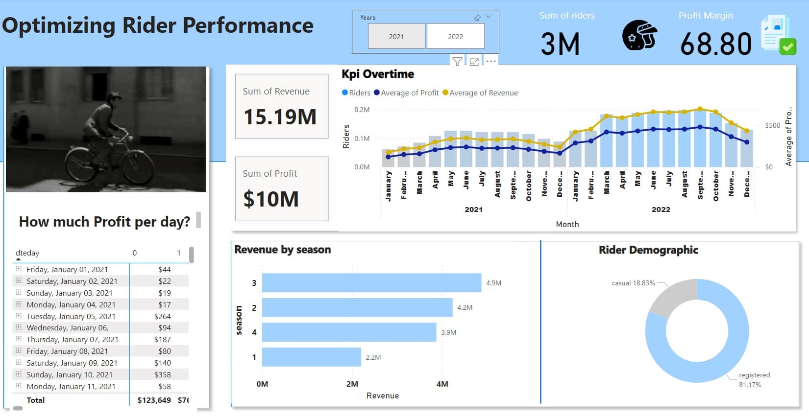
The dashboard surfaces the joined data as: daily profit breakdown, a KPI-over-time view (riders, average profit, average revenue across 2021–2022), revenue by season, and a registered-vs-casual rider split. Headline numbers from the dashboard: 68.80% profit margin, 3 million total riders tracked, and a clear seasonal skew — summer revenue ($4.9M) more than double winter ($2.2M).

Raw hourly ridership (2 years) + cost table (price, COGS per year)
  → UNION ALL (combine years) + LEFT JOIN on cost table
  → Derived columns: Revenue = riders × price, Profit = Revenue − COGS
  → Analytical queries:
      - avg profit by season × hour (optimal operating windows)
      - CASE-based efficiency categorization (High/Moderate/Low)
      - 7-day rolling profit window (trend smoothing)
      - LAG(riders) → previous_day_riders (feature prep, not a model)
  → Power BI dashboard (reads the joined/derived data directly)

Key engineering decisions:

• Derive Revenue and Profit once, in the join, not per-query — computing riders × price and Revenue − COGS as part of the initial join means every downstream query works from the same consistent numbers, rather than each analysis recomputing (and potentially drifting on) its own definition of profit.
• Cost-efficiency as a category, not just a raw ratio — bucketing revenue-to-COGS into High/Moderate/Low efficiency turns a continuous number into something an operations team can act on directly ("focus on the Low-efficiency slots"), rather than requiring everyone reading the dashboard to interpret a raw ratio themselves.
• Rolling window over raw daily numbers — a 7-day rolling profit sum smooths out day-to-day noise (a single unusually good or bad day) so the seasonal trend is visible in the dashboard rather than buried in daily variance.
• Lagged features prepared, not a forecasting model claimed — the LAG() query produces exactly the kind of feature (previous_day_riders) a time-series or regression model would need, but no model was actually trained here. This page names it as what it is: data preparation for a future step, not a delivered prediction.

Actual demand forecasting (e.g., a simple regression or time-series model on the prepared lagged features) and real anomaly detection (e.g., flagging days where revenue or rider count falls outside a statistical band) are natural next steps — the SQL groundwork for both already exists in this pipeline, but neither was built as part of this project.